- and d. The estimated equation is:
                        _          _
   Xi         Yi    Xi - Xn   (Xi - Xn)2    ki
  ---------------------------------------------------
   0         -2       -2         4      -2/10 = -.200
   1         -1       -1         1      -1/10 = -.100
   2          1        0         0          0 =  .000
   3          1        1         1       1/10 =  .100
   4          1        2         4       2/10 =  .200
  ---------------------------------------------------
  10          0        0        10       0/10 =  .000
From the Table:
åi=1,5 ki = 0
åi=1,5 kixi = (-2/10)*0+(-1/10)*1+(0)*2+(1/10)*3+(2/10)*4 = 1
                          _
åi=1,5 ki2 = 1/[åi=1,5 (xi - Xn)2] = 1/10 =
          = (-2/10)2  + (-1/10)2 + (0)2 + (1/10)2 + (2/10)2 =
          = 10/100 = 1/10 = .100
^
b1  = åi=1,5 kiyi
    = (-2/10)*-2 + (-1/10)*-1 + (0)*1 + (1/10)*1 + (2/10)*1
    = (4+1+0+1+2)/10 = .800
^     _   ^ _
b0  = y - b1X = 0 - (8/10)*2 = -16/10 = -1.6
                          ^
   yi  = -1.6 + .800*xi + ei
Which produces the fitted values:
   ^
   yi  = -1.6 + .800*xi
and the estimated residuals
        ^         ^
   ei = ei = yi - yi = yi + 1.6 - .800*xi
This produces the table
                ^              ^                   _
 xi     yi      yi    ei = yi - yi     eixi     yi - y
----------------------------------------------------
 0     -2     -1.6      -.400         0.0       -2
 1     -1     - .8      -.200         -.2       -1
 2      1      0.0      1.000         2.0        1
 3      1       .8       .200          .6        1
 4      1      1.6      -.600        -2.4        1
----------------------------------------------------
10      0      0.0      0.000         0.0        0
-
SSE = åi=1,5 ei2 = -.42 + -.22 + 12 + .22 + -.62 = 1.6
                   _
SSTO = åi=1,5 (yi - y)2 = -22 + -12 + 12 + 12 + 12 = 8

     SSTO - SSE    8 - 1.6
R2  = ---------- = --------- = .8
        SSTO          8
s2 =
[åi=1,5 ei2]/(n - 2) = 1.6/(5-2) = .53333
   ^                    _
s2{b1} = s2/[åi=1,5 (xi - X)2] = .53333/10 = .053333
   ^                                 _
s2{b0} = [s2åi=1,5 xi2]/{n[åi=1,5 (xi - X)2]}
       = (.53333*30)/(5*10) = .31999
Hence:
  ^
s{b1} = .23094
  ^
s{b0} = .56568
The hypothesis test is:Ho: b1 = 0
H1: b1 ¹ 0
Our test statistic has a t distribution with n - 2 = 3 degrees of freedom:
                  ^          ^
test statistic = (b1 - b1)/s{b1} = .800/.23094 = 3.4641
Using EVIEWS, P-Value (two-tail) = .04052.Ho: b0 = 0
H1: b0 ¹ 0
Our test statistic has a t distribution with n - 2 = 3 degrees of freedom:
                  ^          ^
test statistic = (b0 - b0)/s{b0} = -1.6/.56568 = -2.8284
Using EVIEWS, P-Value (two-tail) = .06628.Below is the EVIEWS output. The first three columns of the table contain exactly the same values as those calculated in parts b, f and g respectively. As for the statistics below the table, we found R (R-squared) in part e, s (SE of regression) and the SSE (sum of squared residuals) in part f. The Mean of the dependent variable (Y) can be found in parts b,c or d. The 2 tail significance values below are the same as the ones computed above.
============================================================
LS // Dependent Variable is Y
Date: 03/02/98   Time: 22:21
Sample: 1 5
Included observations: 5
============================================================
      Variable      CoefficienStd. Errort-Statistic  Prob.
============================================================
         C          -1.600000   0.565685  -2.828427   0.0663
         X           0.800000   0.230940   3.464102   0.0405
============================================================
R-squared            0.800000    Mean dependent var 0.000000
Adjusted R-squared   0.733333    S.D. dependent var 1.414214
S.E. of regression   0.730297    Akaike info criter-0.339434
Sum squared resid    1.600000    Schwarz criterion -0.495659
Log likelihood      -4.246107    F-statistic        12.00000
Durbin-Watson stat   1.725000    Prob(F-statistic)  0.040519
============================================================
The results of the simple linear regression are given below:
============================================================
LS // Dependent Variable is FUEL
Date: 03/02/98   Time: 22:29
Sample: 1 8
Included observations: 8
============================================================
      Variable      CoefficienStd. Errort-Statistic  Prob.
============================================================
         C           15.83786   0.801773   19.75353   0.0000
        TEMP        -0.127922   0.017457  -7.327679   0.0003
============================================================
R-squared            0.899489    Mean dependent var 10.21250
Adjusted R-squared   0.882737    S.D. dependent var 1.910451
S.E. of regression   0.654209    Akaike info criter-0.636340
Sum squared resid    2.567934    Schwarz criterion -0.616480
Log likelihood      -6.806148    F-statistic        53.69488
Durbin-Watson stat   3.017045    Prob(F-statistic)  0.000330
============================================================
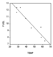
The plot looks like this:
To find a point estimate of the expected value of fuel consumed when the average hourly temperature is 41, we simply plug 41 into our estimated equation:
        ^     ^     ^
        yp  = b0  + b1 xp  = 15.83786 - .127922*41 = 10.593058
The 95% confidence interval for the point estimate in (c) is given by:
^     ^                                   _     ^
b0  + b1 xp ± t.025,n-2[s2(1 + 1/n) + (xp - X)2s2{b1}]1/2
Thus we find15.83786 - .127922*41 ± 2.447*[.6542092(1 + 1/8) + (41 - 43.975)2(.017457)2]1/2
and the confidence limits are: (8.8904, 12.2958)
============================================================
Dependent Variable: DCOUT
Method: Least Squares
Date: 03/03/98   Time: 14:56
Sample: 1 25
Included observations: 25
============================================================
     Variable      CoefficientStd. Errort-Statistic  Prob.
============================================================
         C           0.130875   0.125989   1.038779   0.3097
       WIND          0.241149   0.019049   12.65927   0.0000
============================================================
R-squared            0.874493    Mean dependent var 1.609600
Adjusted R-squared   0.869036    S.D. dependent var 0.652278
S.E. of regression   0.236052    Akaike info criter 0.027090
Sum squared resid    1.281573    Schwarz criterion  0.124600
Log likelihood       1.661381    F-statistic        160.2571
Durbin-Watson stat   0.536610    Prob(F-statistic)  0.000000
============================================================
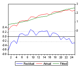
And here is a graph of the fitted function and the residuals:
Below is the EVIEWS output for the paper strength example:
============================================================
Dependent Variable: TENSILE
Method: Least Squares
Date: 03/03/98   Time: 15:17
Sample: 1 19
Included observations: 19
============================================================
     Variable      CoefficientStd. Errort-Statistic  Prob.
============================================================
         C           21.32126   5.430178   3.926439   0.0011
     HARDWOOD        1.770986   0.647814   2.733788   0.0141
============================================================
R-squared            0.305374    Mean dependent var 34.18421
Adjusted R-squared   0.264513    S.D. dependent var 13.77777
S.E. of regression   11.81589    Akaike info criter 7.876068
Sum squared resid    2373.458    Schwarz criterion  7.975482
Log likelihood      -72.82264    F-statistic        7.473597
Durbin-Watson stat   0.246890    Prob(F-statistic)  0.014140
============================================================
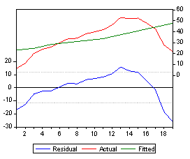
And here is a graph of the fitted function and the residuals: