- In this problem we are going to analyze the nations data
with a more realistic Likelihood Function where we assume that the
observed distances have a log-normal distribution. We are also
going to take a Bayesian approach and state prior distributions for
all of the parameters of our model. Hence, rather than minimizing
a squared-error loss function we are going to maximize the
log-likelihood of a posterior distribution.
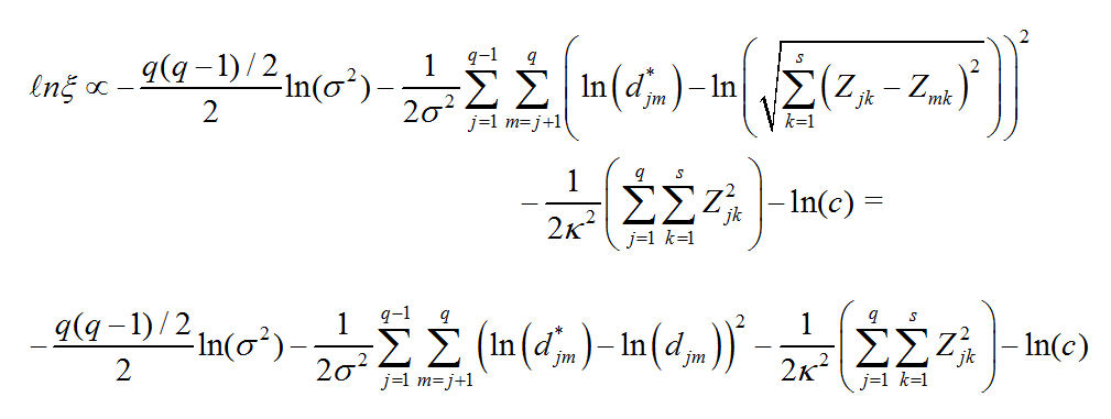
We assume that our observed distances have the log normal distribution:
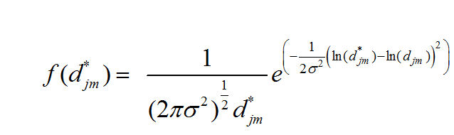
Which produces the Likelihood Function:
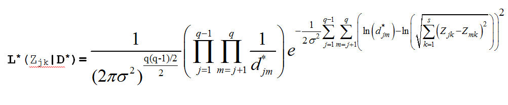
Our prior distributions for the coordinates and the variance are:
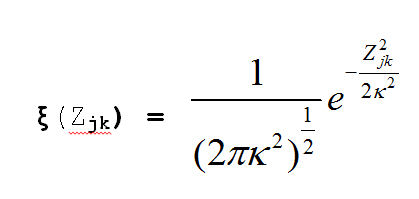
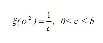
And the log of our Posterior Distribution is:
We are going to use a version of metric_mds_nations_ussr_usa.r which we used in Homework 8, Problem 2 to find the coordinates and the variance term that maximizes the log-likelihood of the posterior distribution.
Download the R program:
 metric_mds_nations_log_normal_2.r
-- Program to optimize the Log-Normal Bayesian Model for the Nations
data.
metric_mds_nations_log_normal_2.r
-- Program to optimize the Log-Normal Bayesian Model for the Nations
data.
Here is the function that computes the log-likelihood:fr <- function(zzz){ # xx[1:18] <- zzz[1:18] xx[21] <- zzz[19] xx[19:20] <- 0.0 xx[22] <- 0.0 xx[23:24] <- zzz[20:21] sigmasq <- zzz[22] We have an additional parameter -- the variance term of the log-normal kappasq <- 100.0 The variance term of the Coordinate priors sumzsquare <- sum(zzz[1:21]**2) Sum of the squared coordinates # i <- 1 sse <- 0.0 while (i <= np) { ii <- 1 while (ii <= i) { j <- 1 dist_i_ii <- 0.0 while (j <= ndim) { # # Calculate distance between points # dist_i_ii <- dist_i_ii + (xx[ndim*(i-1)+j]-xx[ndim*(ii-1)+j])*(xx[ndim*(i-1)+j]-xx[ndim*(ii-1)+j]) j <- j + 1 } Note that this is the sum of squared differences of the logs if (i != ii)sse <- sse + (log(sqrt(TT[i,ii])) - log(sqrt(dist_i_ii)))**2 ii <- ii + 1 } i <- i + 1 } Here we have to include the variance term and the logs of the priors sse <- (((np*(np-1))/2.0)/2.0)*log(sigmasq)+(1/(2*sigmasq))*sse+(1/(2*kappasq))*sumzsquare return(sse) Note that above we have multiplied the log-likelihood by -1 so that the optimizers will find a minimum }The number of parameters is equal to 22 (nparam=22) now and further down in the problem before the optimizers are called zzz[22] is initialized to 0.2.
- Run the program and turn in a
NEATLY FORMATTED plot of the nations.
- Report errordc, xfit,
checkinverse, and rfit.
- Report a NEATLY
FORMATTED listing of the results Table.
- Add the code to produce a graph of the eigenvalues of the
Hessian matrix. Turn in a NEATLY FORMATTED
version of this plot with appropriate labeling.
- Run the program and turn in a
NEATLY FORMATTED plot of the nations.
- In this problem we are going to analyze the famous color similarities data
with the same model we used in problem (1). We assume that the
observed distances have a log-normal distribution. We are also
going to take a Bayesian approach and state prior distributions for
all of the parameters of our model. Hence, rather than minimizing
a squared-error loss function we are going to maximize the
log-likelihood of a posterior distribution. We are going to use a version of
metric_mds_nations_ussr_usa.r
which we used in problem (1) to find
the coordinates and the variance term that maximizes
the log-likelihood of the posterior distribution.
Download the R program:
metric_mds_colors_log_normal.r
-- Program to optimize the Log-Normal Bayesian Model for the Colors Similarities data.
colors.txt
-- Colors Data used by metric_mds_colors_log_normal.r
Here is the function that computes the log-likelihood:fr <- function(zzz){ # xx[1:8] <- zzz[1:8] There are 26 parameters: 14*2=28-3+1=26 xx[9:10] <- 0.0 The 14 points in 2 dimensions = 28 coordinates xx[11:19] <- zzz[9:17] The 5th point -- 490 Angstroms is the origin and xx[20] <- 0.0 the 2nd Dimension of 600 Angstroms is set to 0.0 xx[21:28] <- zzz[18:25] Hence, 25 coordinates plus the variance term = 26 parameters sigmasq <- zzz[26] kappasq <- 100.0 sumzsquare <- sum(zzz[1:25]**2) # i <- 1 sse <- 0.0 while (i <= np) { ii <- 1 while (ii <= i) { j <- 1 dist_i_ii <- 0.0 while (j <= ndim) { # # Calculate distance between points # dist_i_ii <- dist_i_ii + (xx[ndim*(i-1)+j]-xx[ndim*(ii-1)+j])*(xx[ndim*(i-1)+j]-xx[ndim*(ii-1)+j]) j <- j + 1 } if (i != ii)sse <- sse + (log(sqrt(TT[i,ii])) - log(sqrt(dist_i_ii)))**2 ii <- ii + 1 } i <- i + 1 } sse <- (((np*(np-1))/2.0)/2.0)*log(sigmasq)+(1/(2*sigmasq))*sse+(1/(2*kappasq))*sumzsquare return(sse) }The number of parameters is equal to 26 (nparam=26) and further down in the program before the optimizers are called zzz[26] is initialized to 0.2. This program also has much more efficient code for putting the coordinates estimated by the optimizers back into a matrix for plotting purposes:# # Put Coordinates into matrix for plot purposes # xmetric <- rep(0,np*ndim) dim(xmetric) <- c(np,ndim) zdummy <- NULL zdummy[1:(np*ndim)] <- 0 Note the parentheses around "np*ndim" -- R does weird things if you write [1:np*ndim] zdummy[1:8] <- rhomax[1:8] zdummy[11:19] <- rhomax[9:17] I transfer the coordinates from the optimizer back into a vector np*ndim long with the points stacked zdummy[21:28] <- rhomax[18:25] # i <- 1 while (i <= np) { j <- 1 while (j <= ndim) { xmetric[i,j] <- zdummy[ndim*(i-1)+j] Now it is easy to put the coordinates back into an np by ndim matrix j <- j +1 } i <- i + 1 }- Run the program and turn in a
NEATLY FORMATTED plot of the colors.
- Report xfit and rfit and a NEATLY
FORMATTED listing of the results table.
- Add this code fragment from metric_mds_nations_log_normal_2.r:
           #
           InvCheck <- xhessian%*%XXInv
           checkinverse <- sum(abs(InvCheck-diag(nparam)))
           #
and report checkinverse.
- Add the code to produce a graph of the eigenvalues of the Hessian matrix. Turn in NEATLY FORMATTED plot with appropriate labeling.
- Run the program and turn in a
NEATLY FORMATTED plot of the colors.
- In this problem we are going to analyze the famous Morse Code Confusions data
with the same model we used in problems (1) and (2). We assume that the
observed Confusions when transformed to distances have a log-normal distribution. We are also
going to take a Bayesian approach and state prior distributions for
all of the parameters of our model. Hence, rather than minimizing
a squared-error loss function we are going to maximize the
log-likelihood of a posterior distribution. We are going to use a version of
metric_mds_nations_ussr_usa.r
which we used in problems (1) and (2) to find
the coordinates for the letters and numbers and the variance term that maximizes
the log-likelihood of the posterior distribution.
Download the R program:
morse_two_ways_log_normal.r
-- Program to optimize the Log-Normal Bayesian Model for the Morse Confusions data.
morse_confusions_data.txt
-- Morse Confusions Data used by morse_two_ways_log_normal.r
Here is the first part of the function that computes the log-likelihood:fr <- function(zzz){ # # A is set to the origin, (0.0, 0.0) and the 2nd dimension coordinate of # B is set to 0.0 Recall how dissimilar the letters "A" and "B" are # # (26+10)*2 = 72 # 72 - 3 + 1 = 70 There are 70 parameters: 36*2=72-3+1=70 # xx[1:2] <- 0.0 # A xx[3] <- zzz[1] xx[4] <- 0.0 # B 2nd dimension coordinate xx[5:72] <- zzz[2:69] sigmasq <- zzz[70] kappasq <- 100.0 sumzsquare <- sum(zzz[1:69]**2) etc. etc.- Run the program and turn in a
NEATLY FORMATTED plot of the colors.
- Report xfit and rfit and a NEATLY
FORMATTED listing of the results table.
- Add this code fragment from metric_mds_nations_log_normal_2.r:
           #
           InvCheck <- xhessian%*%XXInv
           checkinverse <- sum(abs(InvCheck-diag(nparam)))
           #
and report checkinverse.
- Add the code to produce a graph of the eigenvalues of the Hessian matrix. Turn in NEATLY FORMATTED plot with appropriate labeling.
- Run the program and turn in a
NEATLY FORMATTED plot of the colors.